Time Series Prediction

Time series prediction generates predictions on your dataset given a target and a temporal column.

• Train Time Series. Predict using the Train Time Series skill.
• Univariate Analysis. Prediction with one measure variable.
• Multivariate Analysis. Prediction with one measure variable and one or more variables that affect the measure variable.
• Multiple Time Series. Predictions with multiple measure variables or with one or more grouping variables.
• Group Temporal Repetitions. Adjust datasets with multiple values per temporal variable.

Train Time Series

To Train Time Series, select Machine Learning > Train Time Series in the skill menu.

note

If you're connected to a BigQuery database, you can leverage BigQuery ML within DataChat.

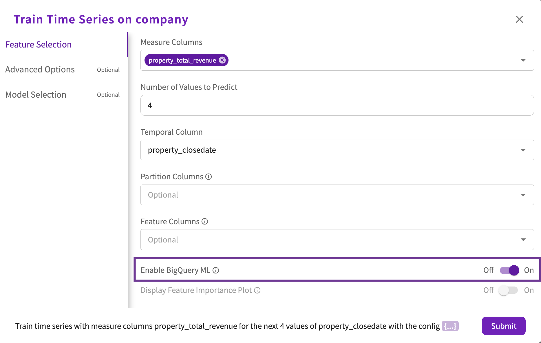
Feature Selection

At a minimum, complete the required fields in the Feature Selection section.

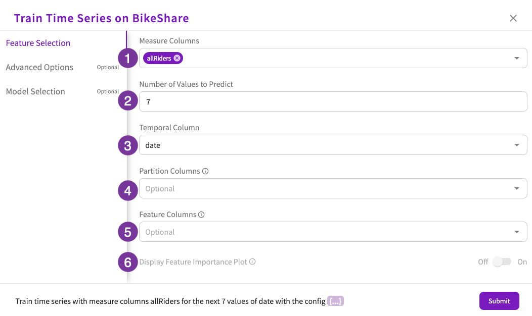
1. Select at least one column that contains measure variables. This is the value you want to predict.
2. Enter the number of values to predict. This is how many steps into the future you want to predict.
3. Select the column that contains your temporal variable.
4. Optionally, select a column that contains a variable that groups your data for better predictions.
5. Optionally, select feature columns to use in your prediction. If any feature columns are selected, the prediction becomes a multivariate.
6. Optionally, choose whether to include a feature importance plot as part of the prediction. Note that this option is only available for multivariate analysis without BigQuery ML enabled.
7. If you're ready, click Submit to run the prediction. Otherwise, refer to the Advanced Options or Model Selection sections for more ways to fine-tune your prediction.

Advanced Options

Optionally, you can change some more advanced settings in the Advanced Options section.

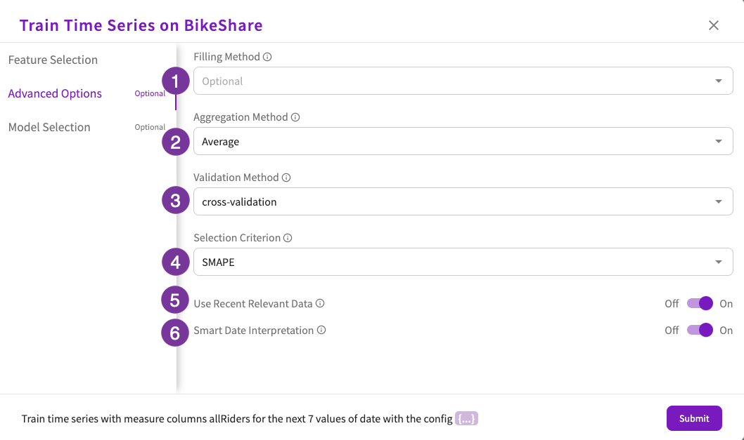
1. Choose the filling method. This is how missing values in the measure or feature columns are handled. The options are:
   • Linear
   • Polynomial
   • Quadratic
   • Spline
2. Choose the aggregation method. This is how duplicate values for a given temporal value are handled. By default, duplicate values are averaged. The options are:
   • Average
   • Maximum
   • Median
   • Minimum
   • Total
3. Choose the validation method. This is how the system validates the model. The options are:
   • Cross-validation
   • Holdout. If this option is selected, you also need to specify the percentage of the dataset that should be held out for validation purposes. By default, 10 percent of the dataset is held out.
4. Choose the selection criterion. This is the scoring criterion that is used to choose the best model. By default, the SMAPE criterion is used. The options are:
   • SMAPE
   • MAE
   • Mean Squared Error
   • Root Mean Squared Error
   • r²
5. Choose whether to use recent relevant data. When selected, the system uses only the 1,000 most recent data points to make a prediction. This can be useful when making long term predictions. This option is enabled by default.
6. Choose whether to use smart data interpretation. When selected, the system interprets string type temporal columns that use the YYYY-MM or YYYY-Q format as datetime columns. This option is enabled by default.

Model Selection

Optionally, select the method to use to predict the values. If no method is chosen, either ARIMA, MLForecast, Prophet, or Theta will be chosen. See here for more information on each method. The options are:

• ARIMA. Uses a statistical model.
• MLForecast. Uses a machine learning model (instead of a statistical model) to optimize your time component for predictions. Note that this method works only for univariate predictions.
• Prophet. Uses a statistical model.
• Theta. Uses a statistical model and is best for short-term predictions.

Each method's hyperparameters can be tuned to your needs.

ARIMA

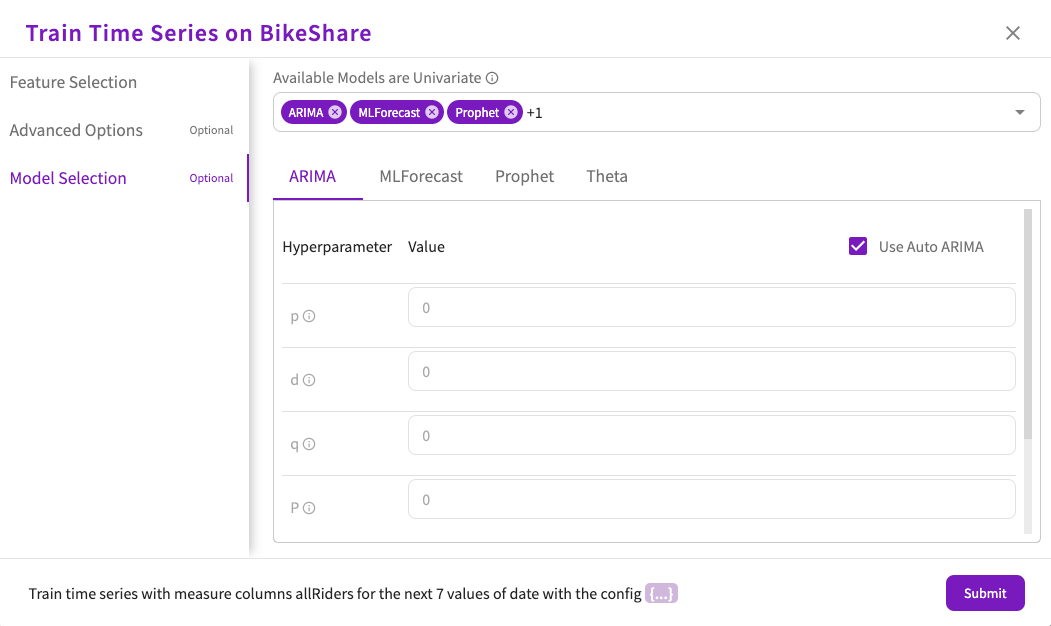
1. Choose whether to use Auto ARIMA, which automatically assigns values for each hyperparameter. If you choose to turn this off, you can then specify your own hyperparameter values.
2. Set a value for the "p" hyperparameter. This parameter determines the non-seasonal autoregression order.
3. Set a value for the "d" hyperparameter. This parameter determines the non-seasonal degree of differencing.
4. Set a value for the "q" hyperparameter. This parameter determines the non-seasonal moving average order.
5. Set a value for the "P" hyperparameter. This parameter determines the seasonal autoregression order.
6. Set a value of the "D" hyperparameter. This parameter determines the seasonal degree of differencing.
7. Set a value for the "Q" hyperparameter. This parameter determines the seasonal moving average order.

MLForecast

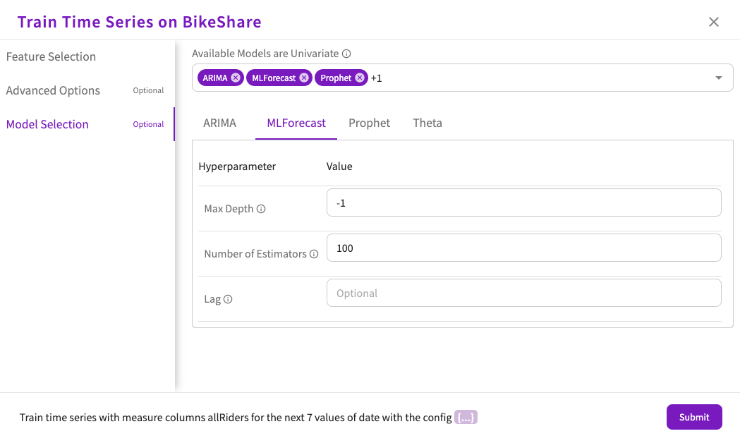
1. Set the value for the Max Depth hyperparameter. This parameter determines the depth of the tree model. By default, this parameter is set to -1, so there is no limit.
2. Set the value for the Number of Estimators hyperparameter. This parameter determines the number of trees in the forest. By default, this parameter is set to 100.
3. Optionally, set the value for the Lag hyperparameter. This parameter determines the number of previous observations to use as features. For example, if this parameter is set to 7 for daily data, then the data in the measure column from a week ago is used.

Prophet

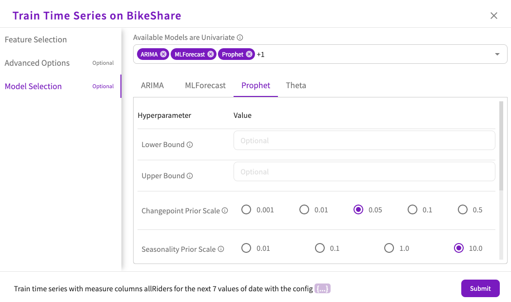
1. Optionally, set the value for the Lower Bound hyperparameter. This parameter determines the lower range of the prediction limit. Note that no models other than Prophet can be selected to change this value.
2. Optionally, set the value for the Upper Bound hyperparameter. This parameter determines the upper range of the prediction limit. Note that no models other than Prophet can be selected to change this value.
3. Set the value of the Changepoint Prior Scale hyperparameter. This parameter determines the flexibility of the model's automatic changepoint selection. A higher values allows for more flexibility.
4. Set the value of the Seasonality Prior Scale hyperparameter. This parameter determines the strength of the seasonality model. A higher values allows for a stronger seasonality model.
5. Set the value of the Holidays Prior Scale hyperparameter. This parameter determines the strength of the holiday model. A higher values allows for a stronger holiday model.
6. Set the value of the Seasonality Mode hyperparameter. This parameter determines the mode used to model the effects of seasonality. The options are:
   • Additive
   • Multiplicative
7. Set the value of the Changepoint Range hyperparameter. This parameter determines the proportion of history in which trend changepoints are estimated.

Theta

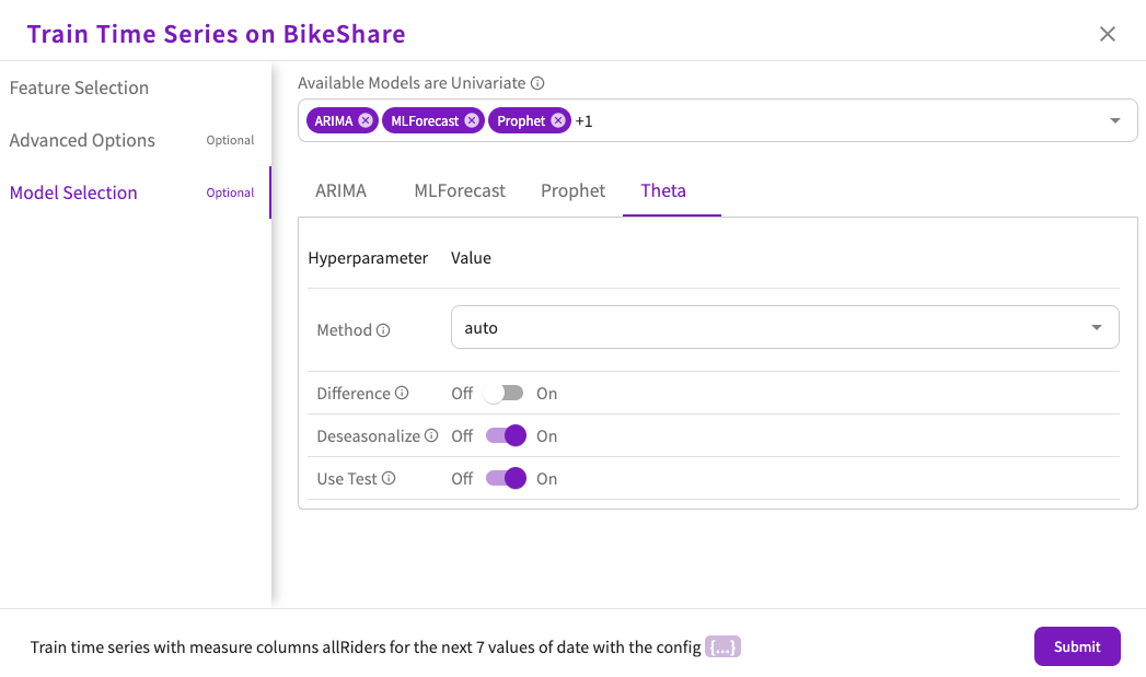
1. Set the value of the Method hyperparameter. This parameter determines the model used for seasonal decomposition. The options are:
   • Auto
   • Additive
   • Multiplicative
2. Choose whether to use the Difference hyperparameter. This parameter determines whether the data is differenced before testing for seasonality. By default, this parameter is off.
3. Choose whether to use the Deseasonalize hyperparameter. This parameter determines whether the data is deseasonalized before forecasting. By default, this parameter is on.
4. Choose whether to use the Use Test hyperparameter. This parameter determines whether the period autocorrelation is tested. By default, this parameter is on.

BigQuery ML

note

For information on BigQuery ML permissions, refer to Database Types.

If your dataset came from a BigQuery connection, you can optionally toggle the Enable BigQuery ML option under Feature Selection, which is enabled by default for BigQuery datasets. When enabled, DataChat leverages BigQuery ML to train time series models.

By default, DataChat explores BigQuery ARIMA Plus models. Optionally, you can specify the hyperparameter types and values under Model Selection:

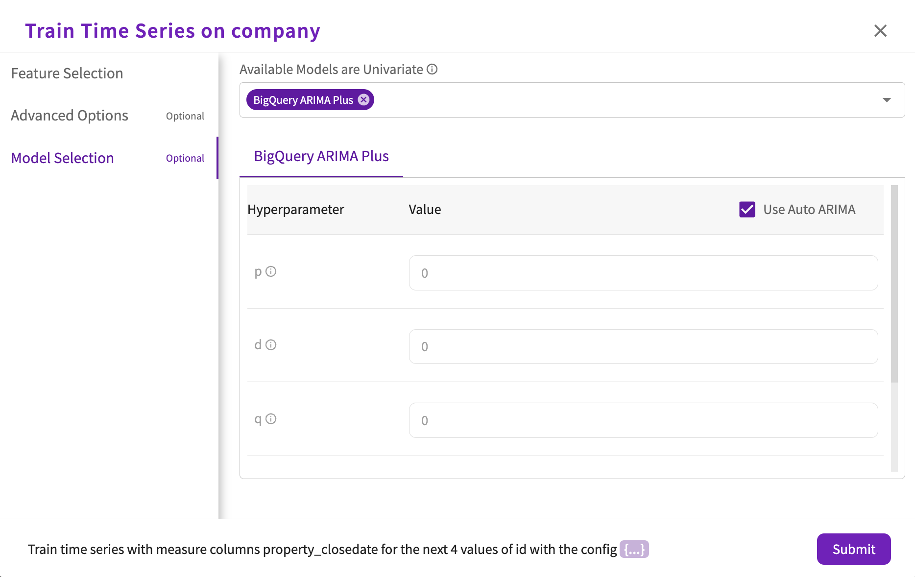
1. Choose whether to use Auto ARIMA, which automatically assigns values for each hyperparameter. If you choose to turn this off, you can then specify your own hyperparameter values.
2. Set a value for the "p" hyperparameter. This parameter determines the non-seasonal autoregression order.
3. Set a value for the "d" hyperparameter. This parameter determines the non-seasonal degree of differencing.
4. Set a value for the "q" hyperparameter. This parameter determines the non-seasonal moving average order.
5. Choose whether to clean spikes and dips automatically. By default, this parameter is set to "true".
6. Choose whether to adjust step changes automatically. By default, this parameter is set to "true".

Outputs

DataChat applies the selected forecasting method (or automatically selects one) to generate the specified number of predicted values for the measure column. A new dataset is created that includes the predicted values. If only one measure variable is specified, the univariate analysis generates a new dataset: PredictedTimeSeries_<measure variable>. If more than one measure variable is specified (multiple time series, which can be either univariate or multivariate) the new dataset is named "PredictedTimeSeries".

note

The current dataset is set to the new, generated dataset. To run a different analysis on the initial dataset, set the current dataset to the initial dataset.

The new dataset is used to generate a chart, which displays in the Chart tab.

note

For charts created with PredictedTimeSeries datasets containing more than 5,000 rows:

• Non-partitioned datasets retain only the most recent 5,000 rows.
• For partitioned datasets, we dynamically allocate historical rows to each partition based on availability, ensuring all forecast rows are fully included and the 5,000-row limit is utilized optimally.

Understand the Available Methods

When predicting time series values, there are four methods available:

• ARIMA
• MLForecast
• Prophet
• Theta

Each method has its own advantages and disadvantages. If you don't manually select a method when using Predict, DataChat looks at your data and decides which method would work best for the prediction. In this section, we'll cover each method in more detail.

ARIMA

The autoregressive integrated moving average (ARIMA) method uses a statistical analysis model with time series data to either better understand the data set or to predict future trends. This method works best with data that has short intervals used for short-term predictions.

Strengths:

• Short-term forecasting
• Needs only historical data

Weaknesses:

• Long-term forecasting
• Predicting turning points

MLForecast

The MLForecast method uses the machine learning regression models instead of statistical models for time series forecasting. It works best with large datasets with well-engineered features.

Strengths:

• Fast and accurate
• Flexible and tunable for accuracy

Weaknesses:

• No confidence intervals
• Performance depends on the size of the dataset and how well the dataset's features were engineered.

Prophet

The Prophet method is a procedure for forecasting time series data based on an additive model where non-linear trends are fit with yearly, weekly, and daily seasonality along with holiday effects. It works best with datasets that have strong seasonal effects and several seasons of historical data.

Strengths:

• Supports forecasting within a range.
• Automatically finds seasonal trends.
• Fast and accurate.

Weaknesses:

• Does not work well outside of seasonal predictions.
• Inputs must be date or datetime values.

Theta

The Theta method is a simple method that uses statistical models to smooth out the data and create predictions.

Strengths:

• Short-term forecasting
• Works with seasonal and stationary data.

Weaknesses:

• Long-term forecasting
• Not as flexible as other methods.

Univariate Prediction

A univariate analysis involves a single measure variable for each time variable. A univariate time series prediction requires:

• At least one measure column that contains target values to predict.
• The number of time intervals to predict.
• One temporal column that contains time interval variables, of date/time type, with one measure variable per time interval.

If DataChat detects repetitions in the temporal columns, you are prompted to aggregate repetitions in the measure variable.

You can use the Train Time Series skill to perform univariate predictions. When training is finished, it provides a number of important results that can be found in the tabbed output:

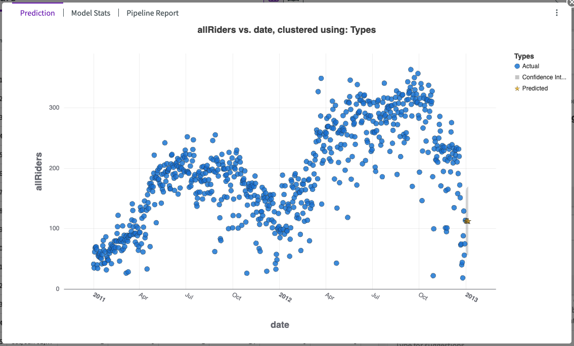
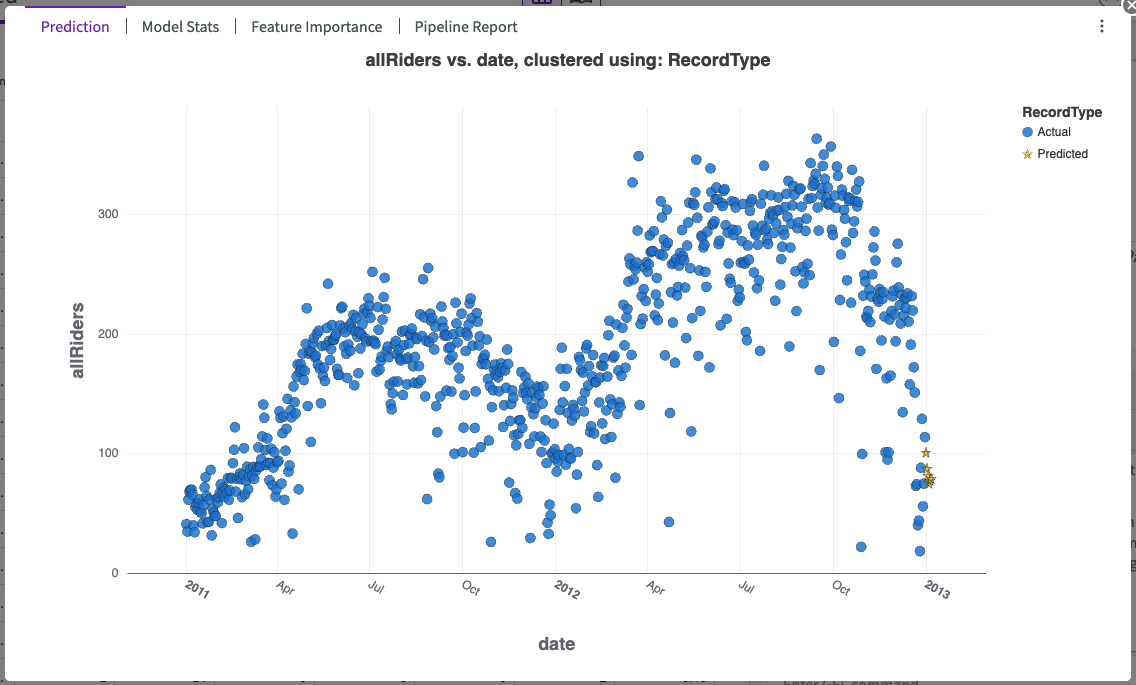
Prediction

The chart's legend shows:

• Data points for the specified measure variable.
• The confidence interval for time series prediction.
• Predicted values for the specified number of time intervals.

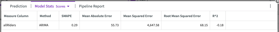
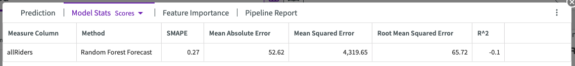
Model Stats

The Model Stats section of Train Time Series output contains two sections:

• Scores
• Model Introspection

Scores

This section displays a table of the model scores to provide context about the success of the prediction model, including:

• Measure Column.
• Method.
• Symmetrical Mean Absolute Error (SMAPE).
• Mean Absolute Error (MAE).
• Mean Squared Error.
• Root Mean Squared Error.
• R². This score is interpreted as the percentage of the data that fits the model's trend. Whether the score is good or bad is highly dependent on the model's use case.

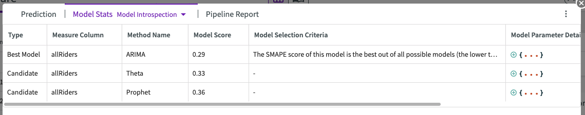
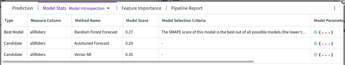
Model Introspection

This section includes a preview for the Model Introspection table. This table provides detailed information about candidate models and their parameters:

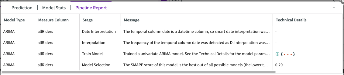
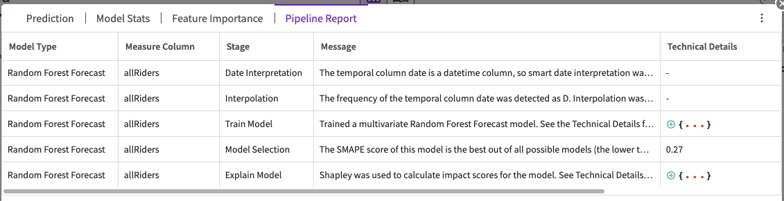
Pipeline Report

The pipeline report shows detailed information about each step of the model training process (known as a “pipeline”). From this report, you can see important information about date interpretation, missing value interpolation, model training, and model selection.

Multivariate Prediction

A multivariate analysis involves at least two variables for each time variable. A multivariate time series prediction requires:

• At least one measure column that contains target values to predict. More than one column generates multiple time series.
• The number of time intervals to predict.
• One temporal column that contains time interval variables, of date/time type.
• At least one column that could influence the measure column.

If DataChat detects multiple measure variables per time interval, you are prompted to group temporal repetitions.

You can use the Train Time Series skill to perform multivariate predictions. When training is finished, it provides a number of important results that can be found in the tabbed output:

Prediction

The chart's legend shows:

• Data points for the specified measure variable.
• Predicted values for the specified number of time intervals.

Model Stats

The Model Stats section of Train Time Series output contains two sections:

• Scores
• Model Introspection

Scores

This section displays a table of the model scores to provide context about the success of the prediction model, including:

• Measure Column.
• Method.
• Symmetrical Mean Absolute Error (SMAPE).
• Mean Absolute Error (MAE).
• Mean Squared Error.
• Root Mean Squared Error.
• R². This score is interpreted as the percentage of the data that fits the model's trend. Whether the score is good or bad is highly dependent on the model's use case.

Model Introspection

This section includes a preview for the Model Introspection table. This table provides detailed information about candidate models and their parameters:

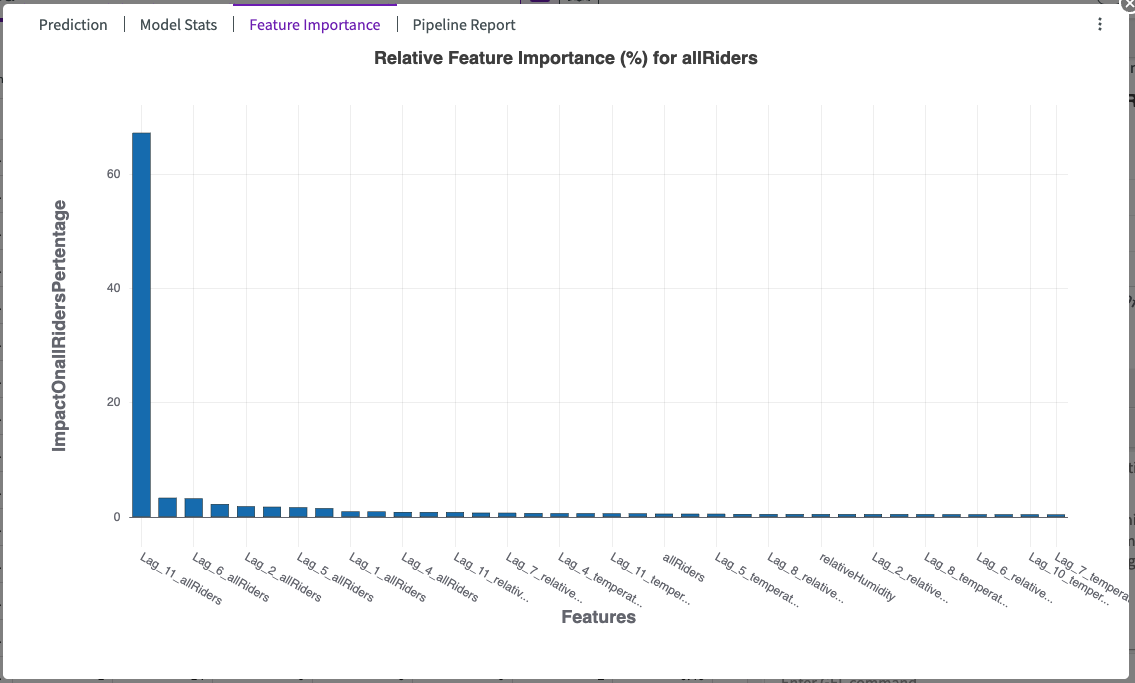
Feature Importance

Training time series on a multivariate prediction produces an impact chart, which illustrates the average impact each input feature has on the target feature. The features are sorted from most- to least-impactful. In the example below, we can see that the “Lag_11_allRiders” feature has the most impact on the “allRidersPercentage”:

Pipeline Report

The pipeline report shows detailed information about each step of the model training process (known as a “pipeline”). From this report, you can see important information about date interpretation, missing value interpolation, model training, and model selection. If enabled, the pipeline report will also explain the model stage, impact scores for each feature column, and lagged features.

Multiple Time Series

You can run multiple time series analyses if you either select more than one measure variable or specify a grouping variable. DataChat runs a separate time series analysis—either univariate or multivariate—for each variable. Every variable must share the same time axis.

You can use the Train Time Series skill to perform both univariate and multivariate predictions.

Examples:

• Generate two univariate trained time series with two measure variables: Train time series with measure columns Bike_North, Ped_North for the next 6 values of Time
• Generate multiple univariate trained time series with a grouping variable: Train time series with measure columns Total_Counts for the next 6 values of Time for each Bike_North
• Generate multiple multivariate trained time series with one grouping variable and another variable that might affect the measure variable: Train time series with measure columns Total_Counts for the next 7 values of Time for each Bike_North using the columns Ped_North

Group Temporal Predictions

If DataChat detects that the column containing your temporal variable has at least one repeated value, meaning that at least two rows contain different measure variables for the same temporal variable, DataChat will prompt you with options to aggregate the measure variables. You can choose by clicking one of the following options, displayed as links:

• Average
• Maximum
• Median
• Minimum
• Total

For each duplicated temporal variable, the measure variables are aggregated as selected in a new dataset called <dataset name>\_Compute>. After you've addressed the repetitions, try your prediction again.