Lending

In this section, we'll investigate bank lending for credit users using a Credit Risk dataset.

Question

Lending analysts have a great responsibility in determining who to lend to. Risky borrowers can cause a number of issues to lenders, including:

• Losing some or all of the principal amount loaned to the borrower.
• Losing revenue from interest and fees.
• Needing to pay more in collection-related expenses such as salaries and attorney fees.
• Experiencing cash flow complications from slow or missed payments.

This leads to a far more difficult question: Which credit applicants are most likely to default?

Challenges

Nearly everyone uses banking, credit, or loans of some kind, leading to a substantial amount of available data, including features such as:

• Whether a customer has made a late payment before.
• How many lines of credit they have.
• The number of dependents they have.

However, despite the availability of this data, several challenges can make analyzing this data complex:

• Technical barriers. Advanced data analytics tools, such as machine learning models and data visualizations may be needed to effectively analyze large amounts of data.
• Interpretations and results. Multiple contextual factors may influence banking behavior, such as the economy, living conditions, profession, and more.
• Bias and error. Interpretation of results can be influenced by individual experience and perspectives.

Method

With DataChat, we can quickly and confidently address these challenges to find meaningful insights in our loan data. We will investigate our dataset, then use our findings to create a model that we can use on future data.

Load Data

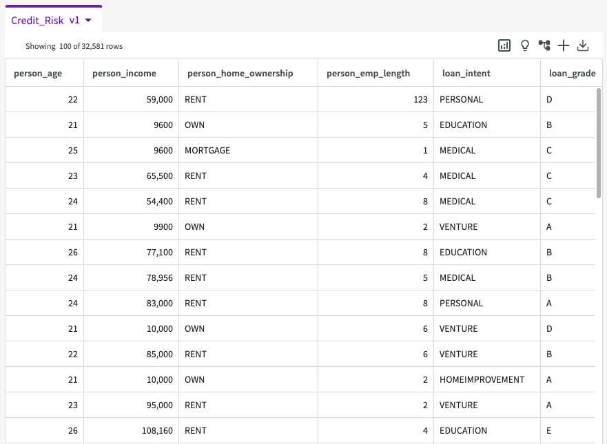
Let's get an idea of the data we're working with. Load the provided demo dataset, "Credit_Risk", into your session. The dataset should look something like this:

Investigate Data

Our dataset includes the following columns:

• person_age. Applicant's age.
• person_income. Annual income.
• person_home_ownership. Type of home ownership.
• person_emp_length. Employment length in years.
• loan_intent. Loan intent.
• loan_grade. Loans graded "A" have the lowest expected risk of loss (low interest rate) while loans graded "G" have the highest expected rate of loss (high interest rate).
• loan_amnt. Loan amount in USD.
• loan_int_rate. Interest rate.
• loan_status. Loan status of "0" (non default) or "1" (default).
• loan_percent_income. Value of the loan compared to applicant's income.
• cb_person_default_on_file. Whether the applicant has historically defaulted.
• cb_preson_cred_hist_length. Credit history length.

From here, we can click Show Descriptive Statistics in the dataset header to provide summary statistics about our data, such as counts, minimum and maximum values, null percentages, and more.

From these statistics we can see that the "Income" column has the largest range in values, from $4000 to $6,000,000. This also reveals that the mean employment length is 4.79 years, the mean loan amount is $9,589.37, and the mean loan interest rate is 11.01%. We can also see certain columns such as "default_on_file", "home_ownership", and "loan_intent" only have between two to six unique response values.

Train a Model

We can now use the Train Model skill to determine which factors most impact whether or not an applicant has defaulted on a loan. Click Machine Learning > Train Model in the skill menu, select "loan_status" for the column, and click Submit. Note that this make take some time. Our impact chart looks something like this:

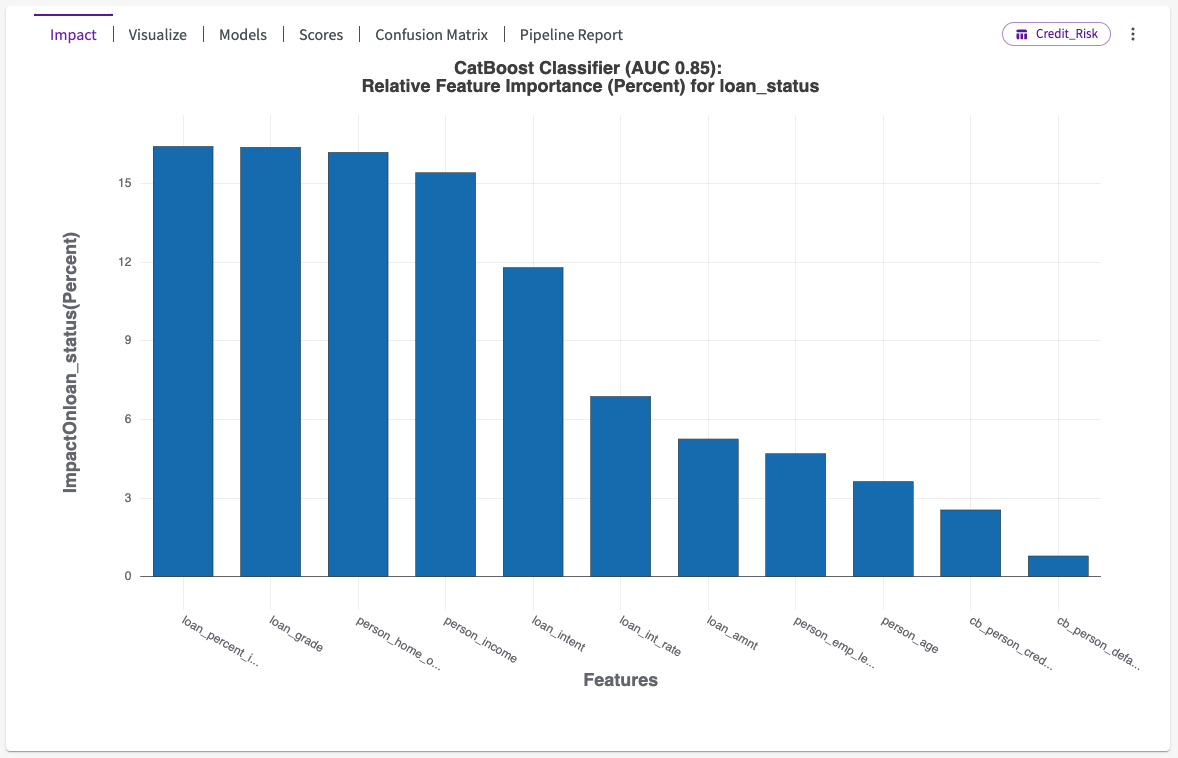
This impact chart shows us five high-impact columns with 85% accuracy: "loan_percent_income", "loan_grade", "person_home_ownership", "person_income" and "loan_intent".

Let's click the Visualize tab from the output, then select Chart1A. This plots seven donut charts that display the loan default status for each loan grade group, "A", indicating low-risk applicants, through "G", indicating high-risk applicants.

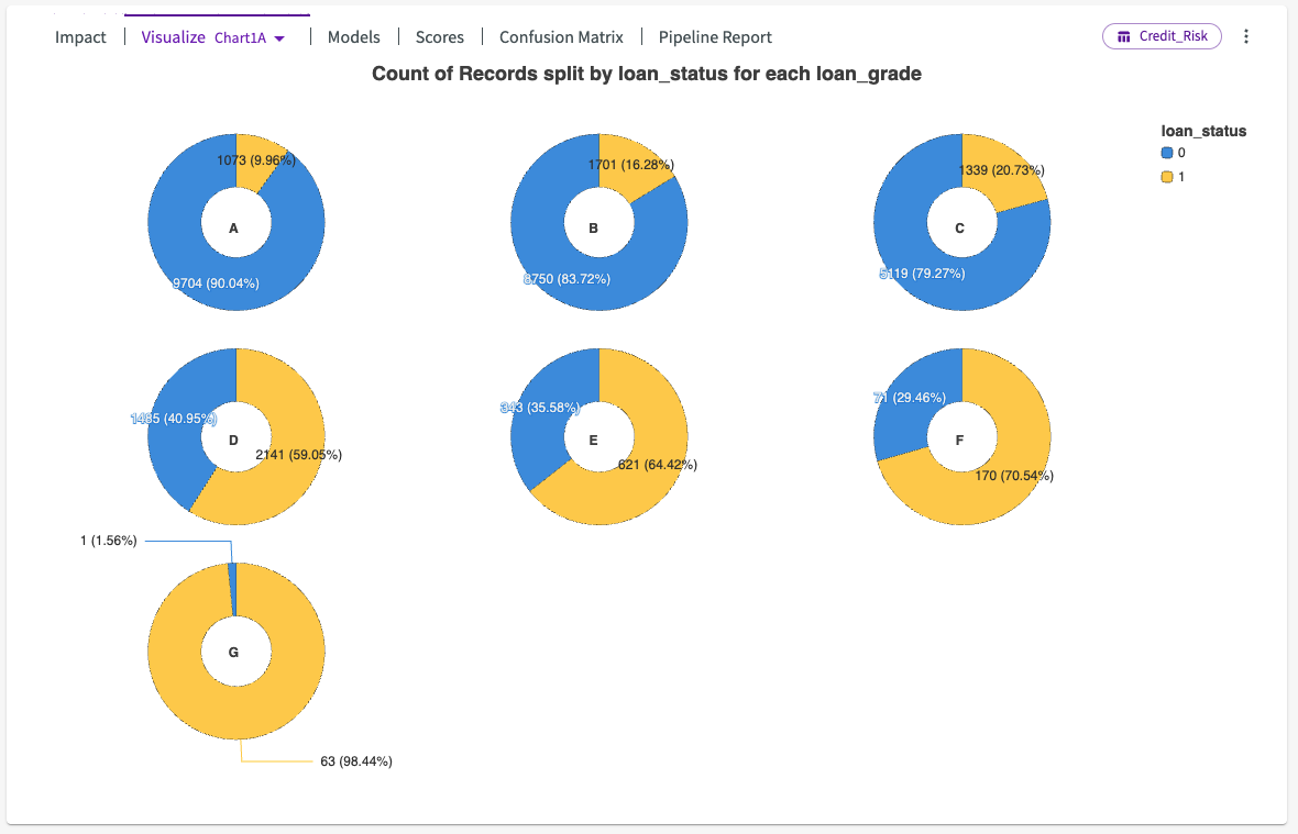
From this chart we can see a direct positive correlation: as risk increases, so does the likelihood that the applicant defaults on their loan.

Let's click on Chart1D. This displays another chart, showing us the relationship between home ownership and loan status for each loan grade.

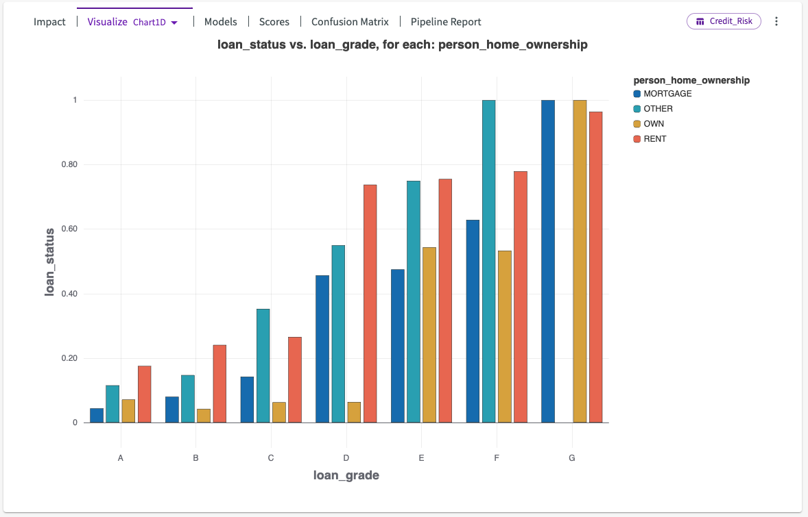
We can see that across all loan grades, renting and "other" (including homelessness and living with family), tend to have the highest default loan status, while owning a home or paying a mortgage tend to have lower defaulting statuses.

Create Visualizations

Let's dive a bit deeper by generating some more visualizations. This will help us to investigate some of the other factors, "loan_percent_income" and "person_income", and how they impact whether an applicant defaults on their loan.

First, let's create a computation that will help us visualize these columns better. Navigate to the Data tab. Click Add Column > Bin in the skill menu, then:

1. Select "person_income" for the column.
2. Select Percentile for the method.
3. Enter "5" for the number of intervals.
4. Click Submit.

Our "person_income" column now has binned intervals by 20th percentiles.

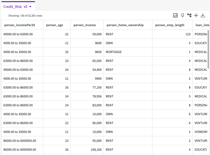
Now we're ready to create visualizations. Click Plot Chart in the skill menu to open the Chart Builder, then:

1. Select "Heatmap" for type.
2. Under Required Fields, select "person_incomePer20" for the X-Axis, "loan_status" for the Y-Axis, and "loan_percent_income" for the Density.
3. Click Submit.

The resulting chart looks like this:

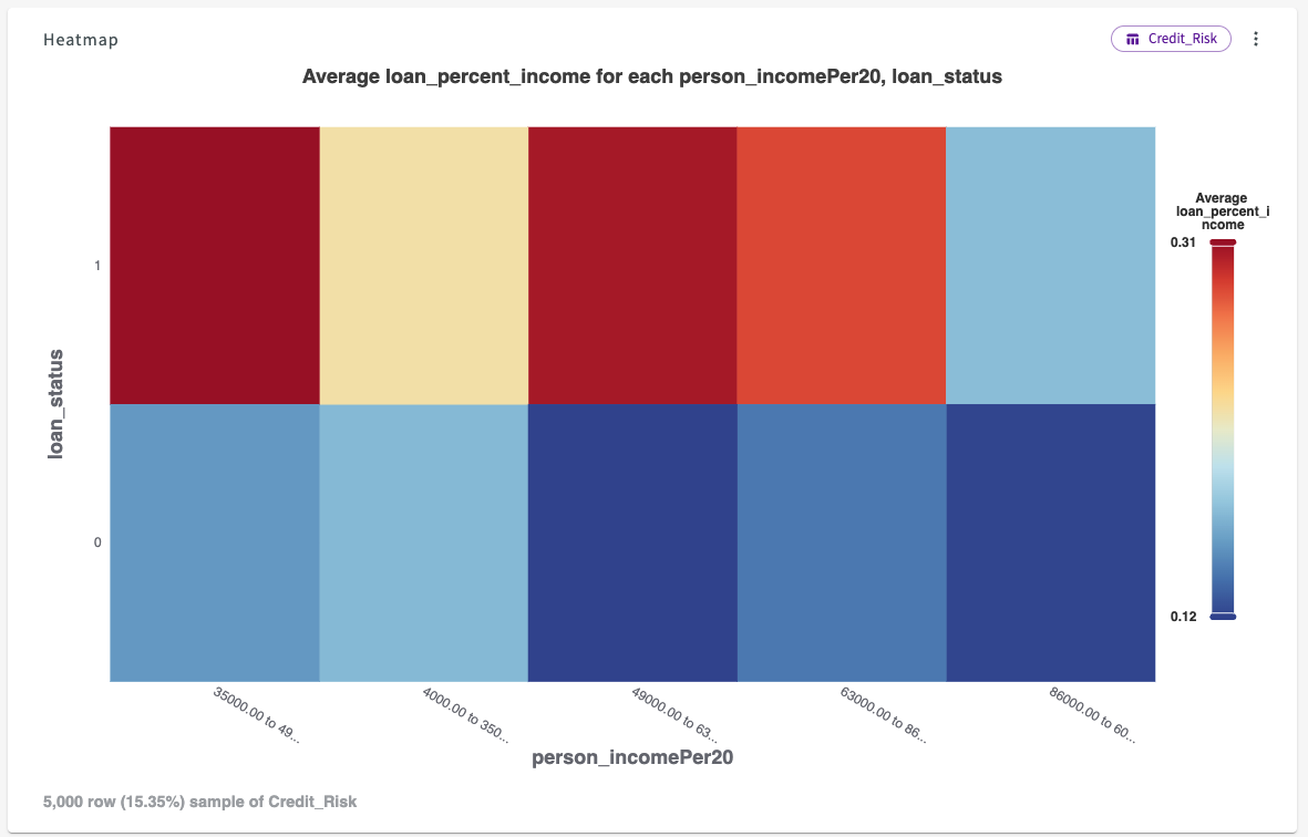
From this chart we can see that as income increases, the average loan value relative to income decreases. Furthermore, the higher the loan value is relative to the applicant's income, the more likely they are to default.

Save a Model

Now that we know the largest impacts on defaulting, let's save this model so that we can use it on future data. This will help to make our lending decisions more efficient in the future.

We can save this model using the Skill form. Click Skill in the skill menu, then enter Save the model BestFit1 as DefaultModel.

When new data is added, we can then Predict using our "DefaultModel" to quickly assess who is likely to default.

Results

Through our analysis, we have identified several factors that most influence whether an applicant is likely to default on their credit:

• The grade of the loan.
• The value of the loan relative to the applicant's income.
• Whether or not the applicant is a home-owner.

We have observed that defaulting on credit decreases as difference in loan amount and income increases, and as loan grade increases. We've also observed that home-owners or those that have a mortgage are less likely to default in comparison to those who rent or are homeless.

Based on these findings, we can recommend several actionable steps to decrease chances of applicant default:

• Use the model, "DefaultModel", when analyzing new applicant data to determine general lending risk.
• Assign higher interest rates to applicants that are likely to default.
• Limit financing options for high-risk borrowers.
• Provide applicants who are rejected information as to how they can improve their chances of credit approval.